Continuing on from the first part of Ben Martins’ investigation in the last issue of CVW, here Ben homes in on the cause of this difficult DAF CF’s repeated cut out.
Wouldn’t it be great if we could identify what the packets of data actually meant or if we could tell which ECUs are online and not?
To begin with, we needed to perform a serial decode on the physical layer to start identifying individual IDs. To do this, click ‘Tools’ > ‘Serial Decode’. You will now have the opportunity to create a decoder by clicking ‘Create’ and selecting ‘CAN’ from the list. The setup box will appear, and you will be asked to select what data you will be decoding. In our case, we will be using A-B, which will be present in the dropdown box. This will only display channels that are active on the grid, so if any have been hidden from view, you will not be able to select them. The next option is to select your threshold. This is the voltage you are telling the software to use as a ‘crossing point’ for the decoder.
Data analysis
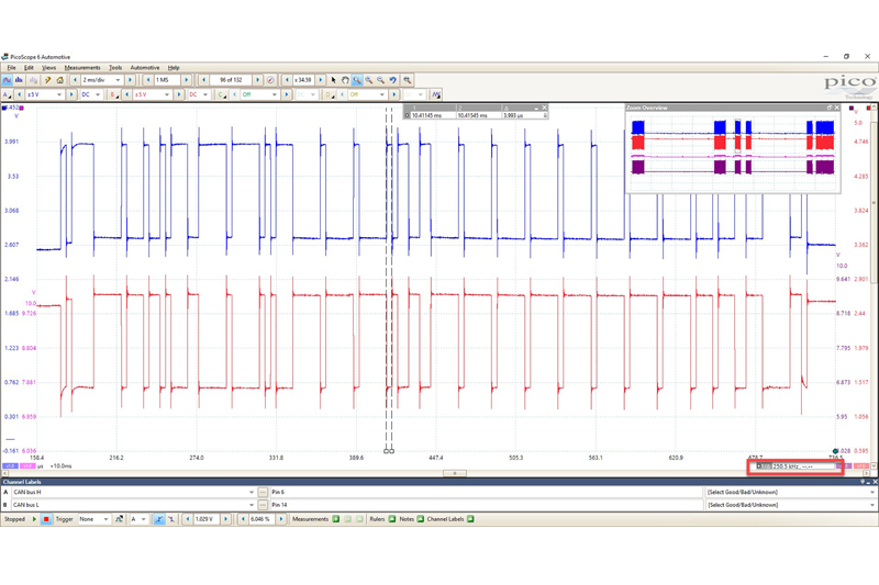
For the purpose of the test, we applied a crossing point of 1V. Hysteresis can come right down to 20mV, as we should be seeing a straight line up and down on our Math channel. The Baud rate can sometimes be a mystery but there is a very simple way of determining what it is by using the time rulers in PicoScope. Using the marquee zoom, draw around a packet of data. Then you can use the time rulers to mark either side of the smallest bit. In the lower righthand corner, you will see a figure in kHz. This will equate to your Baud rate (Fig 1).
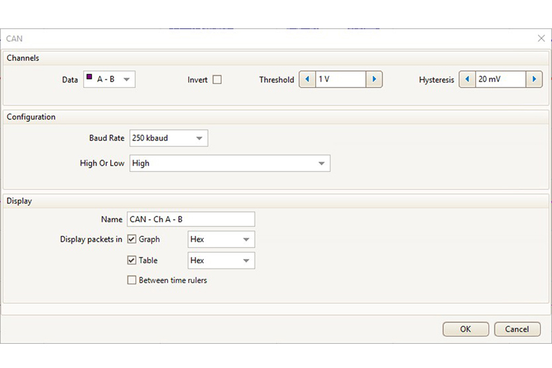
With the settings done, our CAN decode setup should look something like Fig 2.

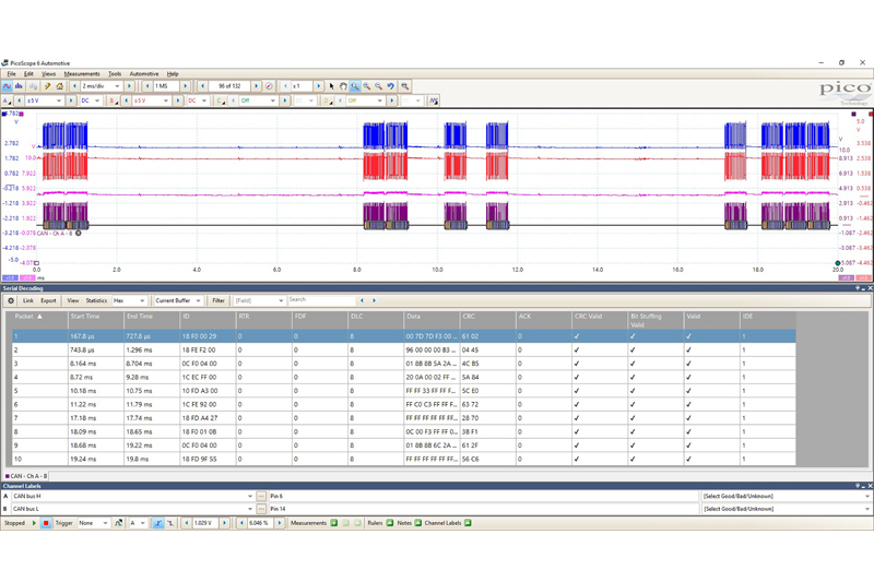
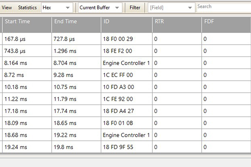
We will now be presented with a table where the packets of data have been converted into HEX code for the current buffer. I purposely selected the buffer just before the first ‘silent’ buffer (with no CAN traffic) as the one to start from as that is where the fault was not present. I have 10 packets of data that all decode correctly with no errors (Fig 3).
Given that J1939 protocol is much more standardised than J2534, we can actually pull this data apart and start identifying IDs. By creating a link file, we can convert the IDs into real words. From our serial data, we had a number of ECUs reporting a problem with the Engine ECM, so it would make sense to look for the Engine ECM ID in our decode table. The first thing we needed to do was to determine which ID is the Engine ECM.
I won’t go into too much detail here, but I do want to show the possibilities that PicoScope can bring when it comes to serial decoding. We must remember, though, that PicoScope is not a dedicated CAN decoder/logger, but an oscilloscope with limited decoder/logger features. That being said, there is still an awful lot we can do.
Cracking the code
To begin with, we need to understand how the message ID of a J1939 message is made up. The message header is made up of 29 Bits, but to keep things simple, we will look at the message in HEX. Each message has a unique Parameter Group Number, PGN, which contains the Suspect Parameter Number, SPN. All we are interested at this stage is the PGN, as this points to a group table that refers to an ECU. To find the PGN in the header, we look to the two middle bytes in an ID, for example – 0C F0 04 00, which means we are only interested in F0 04. We now convert F004 into a decimal, and by using a programmer calculator, we get the number 61444. A quick search through the SAE standards for PGN 61444 confirms to us that this is for the Electronic Engine Controller 1. Therefore, we can be confident that 0C F0 04 00 represented the Engine ECU or EEC1.
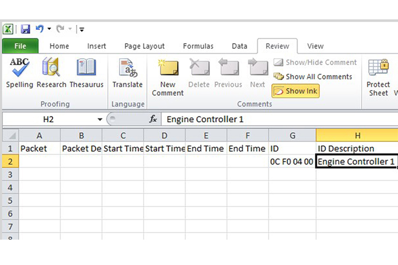
To then apply this to our decode table, we need to fill in this information in our link file and save the file. To get this file, click on the tab in the decode table marked ‘Link’. You will then see an option to ‘Create File’. Once clicked, it will ask you to save a CSV file. Select an appropriate location and then locate and open the saved CSV file. With the file open, there are a number of fields available that look like the decode table in PicoScope but with the additional ID Description header. Copy the ID from PicoScope exactly as it is in the decode table and add the description in the ID description column. For us, this was Engine Controller 1. Make sure you save any changes (Fig 4).
To tell PicoScope to look at this link file and replace any IDs with the description we have listed in the link file, click ‘Link’ > ‘Open’, navigate to the link file location and select. Once selected, you should now see the IDs replaced with a language we can understand (Fig 5).
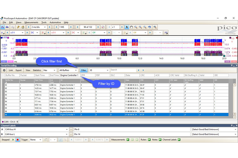
As luck would have it, it was the engine ECU we were looking for. Now we could sort through the data and look for this ID and any faults associated with it. We expanded the decoder to every buffer by selecting ‘All Buffers’ in the dropdown box where the current buffer was selected. We could now export all this data to Excel for further analysis, or we could use the filteroption in the decode table. Select ‘Filter’ and then type the ID you would like to display, which for us was Engine Controller 1 (Fig 6).
We knew the fault occurred at buffer 96, so we started the search from there. Wenoticed that Engine Controller 1 was no longer present after buffer 96, and it appeared to have gone offline despite this ID being very active throughout every buffer previous in the capture. Could this mean that the Engine ECU was at fault? It would make sense and we certainly had proof with our raw CAN Data. We could see that after buffer 96, something happened; the network was silenced, and from here on out the engine ECU was no longer online. This gave us enough reason to send the ECU away for testing, and sure enough, it was confirmed as faulty. A new Engine ECU was fitted, coded and reprogrammed, and the vehicle was back on road.
This was an intriguing case and one that could have been costly for both the owner and us with the wrong diagnosis, but thanks to the PicoScope, we had enough evidence to justify the path we took with the repair.